Algorithms at the Edge AI

In the previous post, we learned about the processors at the edge. In this post, we will try to understand the algorithms at the Edge, differentiating them by their usage, strength, weakness, and suitability for the Edge. There are two major categories of algorithms, feature engineering and artificial intelligence. Feature engineering is primarily playing with the data so that it can be passed on for analysis. Algorithms are what work on the data.

Feature Engineering

Feature engineering is the process of taking raw data and converting it into inputs for statistical tools. These tools describe model situations and processes. Domain understanding is needed to know which parts of the raw data are relevant information.

In the case of Edge AI, we would deal with a lot of time series-based sensor data. Feature engineering would be extracting value out of this sensor data. The time series data must be cut into chunks to process the data. One such chunk is called a window. The number of windows that can be processed in a second is called the frame rate. The window size could be chosen so that the windows fall in sequence or overlap. When the windows overlap, the chances of missing an important signal are low but you might be processing extra information.

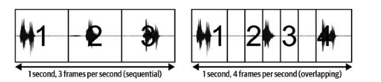
If there is a gap between the windows, relevant information or events might be lost. Deciding the window size and frame rate are important considerations; they are inversely proportional. A large window size would reduce the frame rate, and a Smaller window size would increase it.

DSP (Digital Signal Processing) Algorithms

DSP Algorithms help digest the information from the sensors. Following are some of the DSP algorithms

a. Resampling – All time series signals have sample rate (frequency) i.e. the number of data samples per second in one frame. Downsampling may be needed if it produces more data than can be processed. It involves throwing away some samples of data. For example, if the current frequency or sample rate is 15 samples per second and you throw 2 out of every 3 frames, you effectively get 15 samples in 3 seconds; hence, the sample rate is 5 Hz instead of 15 Hz. In most edge AI use cases, downsampling is required to process data.

In some cases, upsampling might be needed, where extra samples are synthetically introduced each second. The added sample data is an approximation of the data as it comes in, which is called interpolation. Upsampling is usually applied when we want to mix 2 signals in the same time series for analysis.

b. Filtering – It is a transformation function. Low-Pass Filters – Allow low-frequency elements of the filter to pass through and remove the high-frequency elements. Cutoff frequency defines the frequency beyond which the signal would be left out. The High-Pass filter does the opposite. All frequencies apart from the band pass (125 Hz to 8 kHz) are rejected in speech-to-text recognition. A low-pass filter smoothens out data and a high-pass filter sharpens data.

c. Spectral analysis – Change in frequency over time is shown as

and how much of the signal lies in various frequency bands over a range of frequencies (Spectrogram)

The most common algorithm to convert from the time domain to the frequency domain is the Fourier transform.

d. Image Feature Detection – This is a subset of signal processing algorithms concerned with extracting useful information from the images. Some common examples are edge detection (identifying boundaries), corner detection, Blob detection (identifying regions with commonality), and Ridge detection (identifying curves in images). OpenCV and OpenMV provide a set of libraries for feature detection of images.

Feature scaling is a concept in which instead of passing a lot of extreme scale features to a machine learning model, the features are normalized by rescaling. That means identifying minimum and maximum values for a specific feature in a representative sample. The normalized value is then calculated with

normalized_value = (raw_value - minimum) / (maximum - minimum)

This is done to allow the machine learning models to work with good results rather than having features at wildly different scales. This allows the machine learning algorithms to create a valid data set to learn from, ignoring the wild swings.

Artificial Intelligence Algorithms

(I) By Functionality – What they are designed to do

a. Classification – Distinguishes various types or classes of things like fitness algorithms with the help of an accelerometer, can distinguish between running and walking. An image algorithm with the help of a visual sensor can tell if a container has space or is full. Classification can be binary (one of two classes), multiclass (belongs to one or more classes), multilabel (belongs to zero or more classes)

b. Regression – These algorithms try to come up with numbers. Based on historical information, what temperature would be of the machine in the next hour? A virtual sensor that tries to estimate the speed of the motor based on its sound. Virtual sensors are interesting because they can predict the data for a sensor that is not present by using the data feed of a sensor that is present. Like estimating the speed with sound.

c. Object detection and segmentation – As the name suggests, it is used to identify objects in an image or a video. It puts a box around them. It works in conjunction with classification and regression algorithms.

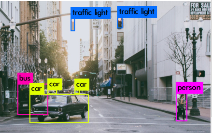
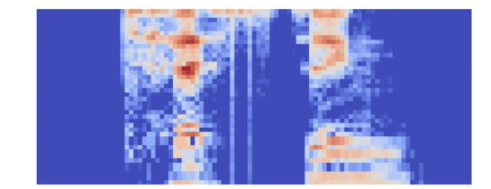
Segmentation algorithms classify images at the pixel level. Different parts are shown in different shades.

d. Anomaly Detection – Recognise when the signal deviates from its normal behavior. They are useful for predictive maintenance. For example, if the motor breaks down soon based on its current draw, the vacuum knows that it is on a different kind of surface using its accelerometer.

e. Clustering – Groups inputs by similarity and would know if the input is not similar to what it has seen before. Identifying the normal state of a machine, the normal voice of a human, and recommendation algorithms based on what the user likes

f. Dimensionality Reduction – These algorithms take a signal and produce an output that contains equivalent information but takes a lot less space. Like compression algorithms for audio, data, etc. The original signal and compressed signal can be compared with each other as well to know that the compressed signal is from the original, like facial recognition or fingerprint recognition.

g. Transformation – Take in one kind of signal and produce a different kind, either related to the original signal or completely different. For example, taking input from a dark feed and adding light, and colors to it, like night vision, noise-cancelling headphones filtering out the noise, or speech-to-text that takes in an audio signal and produces words.

(II) By Implementation – How do they work

The functionality of an algorithm tells us what it does. The way it is implemented is important to understand which implementation should be used in the use case from an engineering perspective.

a. Conditionals & Heuristics—The simplest algorithms are conditional based on if conditions. Some of the most popular and widely used ML algorithms based on decision trees are if statements under the hood. Conditional logic is connected to Heuristics. A heuristic is a rule on the basis of which either an action is taken or not. For example, in thermostat systems, the heuristic is the temperature number beyond which the machine might fail. This heuristic might be known after a lot of research, and it needs domain knowledge and historical data inputs.

For example, for predictive maintenance, the known heuristic is that it makes a certain sound before it starts to break down. When the machine is working, its sound characteristics are fed into a frequency domain using the Fourier transform and compared. If it is noticed that the machine might be getting into the area of breakdown, then an alert is issued.

The problem with conditionals and heuristics is the possible combinatorial explosion. There just might be a lot of conditions possible (like the game of chess) and it might not be possible for the algorithm to consider all possible options.

b. Classic Machine Learning – In these algorithms, instead of handcrafting the conditional logic on our own, we train the algorithm with large quantities of data and the algorithm discovers its own rules based on this training data. The ML algorithm builds a model based on the data. This is called training. Once trained, when we run data through this model to make predictions, it is called inference.

Usually, the training is done on the servers before the model is deployed on the Edge. The inference happens on the Edge

Supervised learning is when an expert labels the dataset, and unsupervised learning is when the algorithm identifies the data without human intervention. The biggest drawback of ML algorithms is that they work well with the type of data that they have been trained on. If we pass out-of-distribution input, then it might result in an incomprehensible output. ML algorithms that lend themselves to explainability (i.e. humans can comprehend the results) are better.

Some supervised ML algorithms are

• Regression analysis – learn the mathematical relationship between input and output to predict a continuous value
• Logistic regression – learns the relationship between the input and categories of output
• Support vector machine – learns complex relationships between input and output. Hard to train.
• Decision trees and random forests – Iterative process of if statements to predict an output category or value
• Kalman filter – predicts the next data point given a history of measurements

Some unsupervised ML algorithms are

• Nearest neighbors – Classifies data based on its similarity to known data points
• Clustering – learns to group inputs by similarity

There are hundreds of ML algorithms available. The art and science is to figure out which one to use to get the best results for the use case

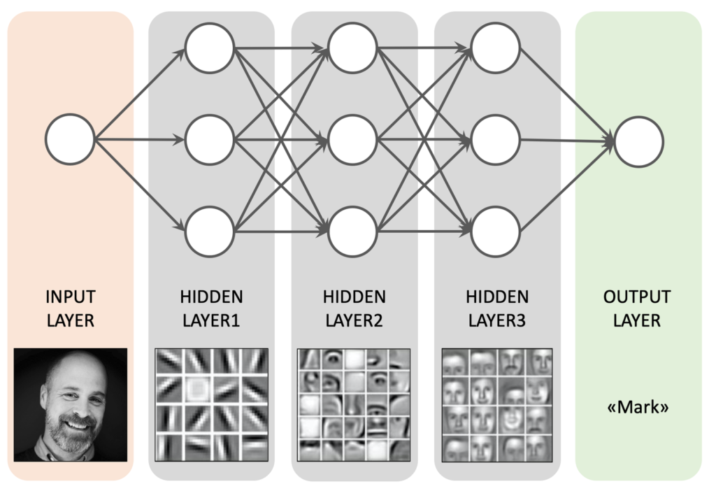
c. Deep Learning – is a type of machine learning that uses neural networks. They are similar to classical ML and a dataset is used to train the model. It is a combination of algorithm + collection of numbers + model’s input to get the output. These numbers are called weights or parameters and are generated during the training process. Neural network refers to how the model combines the inputs with the parameters, this is inspired by how neurons in the brain connect.

AlphaGo, GPT-x, DALLE, and CoPilot are examples of deep learning algorithms.

Deep learning models are effective because they work as Universal Function Approximators. That means that if we can describe anything as a continuous function, i.e. y =f(x) then a deep learning network can model it. In this case, for every x and y, there is a deep learning model that can convert from one to another. An interesting characteristic of this is that during training, the deep learning model can do its feature engineering, i.e. if a special transformation is needed to convert input to output, then it can learn how to do it. The reason they are so good at approximating functions is that they have a large set of parameters, with each parameter, they get a little more flexibility to describe a slightly more complex function.

Deep learning models have 2 kinds of drawbacks. One is their need for a large set of parameters. This involves training with a lot of data, and it can be hard to find data. Next is overfitting. Due to large learning data sets, the deep learning model learns the data too well and hence responds under that data only and falters when it sees any other data.

Some deep learning models are

• Fully connected models – They have a stacked layer of neurons. The input is fed in as a long series of numbers. They are capable of learning any kind of function. They work well with discrete data sets but not with raw time series or image data. Don’t work with spatial data like images.
• Convolutional models – Work with spatial information. Recognize images or structure of signals within time series sensor data.
• Sequence models – recognize long-term patterns in time series data. Work well with spatial data. Might be used as a better alternative for convolutional models.
• Embedding models – Used for dimensionality reduction. Takes a messy input and defines it in a set of numbers that describes that input in a particular context. They are used in image processing, speech recognition, etc. They can be fully connected, convolutional, or sequence models.

Deep learning models are flexible and modular. They consist of layers and operations that can be stacked and combined in an infinite number of ways.

Different arrangements of these layers and operations are called architectures. MobileNet / EfficientNet are family of architectures for mobile devices. YOLO is a family of architectures to perform object detection. Transformers are a family of architectures to translate between sequences of data.

Deep learning models are often large and need significant computation power. With the advent of high-end MCUs (with hardware features like SIMD instructions that can run TensorFlow lite) and SoCs (have full OS and interpreters like TensorFlow Lite are used here), it has become possible to install deep learning models on edge devices.

Core advantages of deep learning models are their flexibility, reduced need for feature engineering, and ability to make use of large amounts of data given the high parameter count. They can approximate complex systems and go beyond simple predictions. These models can play games, and generate art and music. However, they do have high data requirements and a propensity towards overfitting.

d. Combining Algorithms – Algorithms can be combined as per the use case in the following formats

• Ensemble – multiple ML models passed the same input. Each has its strengths and weaknesses, and the combination of the results is more accurate than the individual model.
• Cascade – ML models in a sequence. The output of one is fed into another. The heavier and more expensive models are not activated until necessary inputs come from the earlier models in the pipeline.
• Feature extractors – These are pre-trained feature extractors that can be plugged as an input into the model. The model needs to learn only to interpret the output returned by the feature extractor rather than undergo the whole extraction process by itself.
• Multimodal models – these take input from multiple types of data simultaneously, like accepting audio and accelerometer data together.

Optimization for Edge Devices

It is a tradeoff to find the right balance between Task Performance and Computational Performance. How well does the model perform its task, and how much memory and computing does the model need? This is specifically important for Edge devices as they are computationally constrained. They are designed to save on cost and energy and not to maximize computing. Some factors that might help are

Choice of algorithm

Constraints of the target hardware guide the choice of the algorithm. Classic ML algorithms are smaller than deep learning algorithms. Other optimization techniques are to reduce the complexity of feature engineering so that there is less math, reduce the amount of data that reaches the algorithm for processing, reduce the size i.e. weights and layers in case of deep learning models, and choose models that have accelerator support on the device.

Compression & Optimization –

• Quantization – Reducing the amount of precision for numeric representations while still keeping the information that they contain. Instead of using 32-bit floating point reduce it to 8-bit integers where possible. Integer calculations are faster and more portable than floating-point math. It is a lossy optimization that reduces the throughput performance but increases the compute performance.
• Operator fusion – Evaluate operators and see if some of them can be combined into a single fused operator. This is lossless optimization without reduction in task performance, but may only be available for certain combinations of operators
• Pruning – a lossy technique applied during training or a deep learning model. Many models’ weights are put to zero, thus creating a sparse model. Helpful when models need to be sent over the air.
• Knowledge distillation – a lossy deep learning technique where redundancy of weights in a deep learning model is reduced to create a smaller model that performs as well.
• Binary Neural Networks (BNNs) – Similar to quantization where every weight is a binary number. Lossy but fast.
• Spiking neural network (SNNs) – Signals transmitted through the network have a time component. Lossy and need specialized hardware in the form of an accelerator

Model compression has 2 major downsides. One it may need specialized hardware and software to run. This limits the devices it can be used on. Second, due to the lossy nature, it introduces biases and gaps in the model and hence there is a subtle degradation in the predictive performance.

On-Device Training

Generally, models are trained before they are deployed on the device since training needs lots of computation and large amounts of data annotated with labels. In some scenarios, on-device training makes sense

• Predictive maintenance – A small on-device model is trained to understand the normal state of the device. The assumption here is that abnormal states are rare. If that is not the case, the on-device model would not be able to distinguish the normal state from the abnormal state.
• Personalization – Bio authentication data used by end devices like smartphones, which are personal to the user. Here, the data is stored locally on the device and needs to be trained on the device. Here, embedding models convert raw data into numeric representations. The Euclidean distance between the embeddings corresponds to the similarity between two embeddings
• Implicit Association – Here labels are available by association like when the user would be using their device and when they would charge it. This allows for optimized battery charging to improve the battery lifespan of the device. This data is available and stored locally as per the usage habits of the user.
• Federated learning – way of training a model across multiple devices while preserving privacy information. Partially trained models are combined and distributed back to devices. Computationally expensive and involves moving lots of data. The training process is complex as it involves servers and devices, and since multiple devices are involved, there is a chance for security breaches as well.